单个神经元结构

bp1

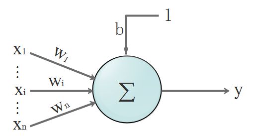
输入：$x_1,x_2,…,x_n$
输出：$y$
输入和输出的关系(函数)：$y = (x_1\ast w_1+x_2\ast w_2+…+x_n\ast w_n+)+b = \sum_{i=1}^n x_i\ast w_i+b$，其中$w_i$是权重
将输入用矩阵表示：$X = [x_1,x_2,…,x_n]^T,X为一个n行1列的矩阵$
将权重用矩阵表示：$W=[w_1,x_2,…,w_n]$
那么输出可以表示为：$y=[w_1.w_2,…,w_n] \cdot [x_1,_2,…,x_n]^T+b=WX+b$

激活函数

激活函数是一类复杂的问题，为便于理解这里有几条重要的特性：

非线性：即导数不是常数，不然求导之后退化为直线。对于一些画一条直线仍然无法分开的问题，非线性可以把直线掰弯，自从变弯以后，就能包罗万象了。
几乎处处可导：数学上，处处可导为后面的后向传播算法（BP算法）提供了核心条件。
输出范围有限：一般是限定在[0,1]，有限的输出范围使得神经元对于一些比较大的输入也会比较稳定。
非饱和性：饱和就是指，当输入比较大的时候，输出几乎没变化了，那么会导致梯度消失！梯度消失带来的负面影响就是会限制了神经网络表达能力。sigmoid，tanh函数都是软饱和的，阶跃函数是硬饱和。软是指输入趋于无穷大的时候输出无限接近上线，硬是指像阶跃函数那样，输入非0输出就已经始终都是上限值。关于数学表示**传送门** 里面有详细写到。如果激活函数是饱和的，带来的缺陷就是系统迭代更新变慢，系统收敛就慢，当然这是可以有办法弥补的，一种方法是使用交叉熵函数作为损失函数。ReLU 是非饱和的，效果挺不错。
单调性：即导数符号不变。导出要么一直大于0，要么一直小于0，不要上蹿下跳。导数符号不变，让神经网络训练容易收敛。

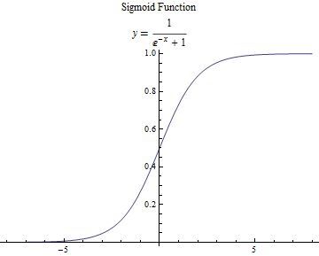
这里用到Sigmoid函数方便理解：

Sigmoid函数：$$y = \frac{1}{e^{(-x)}+1}$$

bp2

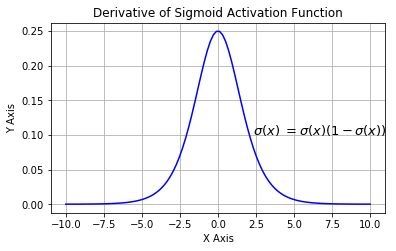
S函数的导数：

$$
\begin{aligned}
&y’= (\frac{1}{e^{-x}+1})’ \\
&=(\frac{u}{v})’,这里u=1,v=e^{-x}+1 \\
&=\frac{u’v-uv’}{v^2} \\
&=\frac{1’\ast (e^{-x}+1)-1\ast (e^{-x}+1)’}{(e^{-x}+1)^2} \\
&=\frac{e^{-x}}{(e^{-x}+1)^2} \\
&=\frac{1}{1+e^{-x}}\ast \frac{1+e^{-x}-1}{1+e^{-x}} \\
&=\frac{1}{1+e^{-x}}\ast (1-\frac{1}{1+e^{-x}}), 令y=\frac{1}{e^{-x}+1} \\
&=y\ast (1-y)
\end{aligned}
$$

S函数的导数的图像：

bp3

传播过程

下面是一个典型的三层神经网络结构，第一层是输入层，第二层是隐藏层，第三层是输出层。

bp4

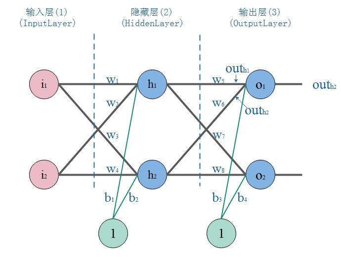
正向传播：输入$i_1,i_2$数据，然后一层一层传播下去，知道输出层输出结果。
反向传播：输入、期望的输出为已知。在开始时，权重$w$,偏置$b$初始化为随机值，按网络计算后观察结果。根据结果的误差(也叫损失)，调整权重$w$,偏置$b$，这时就完成了一次反向传播。
当完成了一次正反向传播，也就完成了一次神经网络的训练迭代，反复迭代，误差越来越小，直至训练完成。

BP算法推导和数值计算

初始化参数

输入：$i_1=0.1,i_2=0.2$
输出：$O_1=0.01,O_2=0.99,(训练时的输出期望值)$
权重：$ \begin{aligned} &w_1=0.1,w_2=0.2,w_3=0.3,w_4=0.4 \\ &w_5=0.5,w_6=0.6,w_7=0.7,w_8=0.8 \\ &(这些权重是随机初始化的，通过多次迭代训练调整直到训练完成)\end{aligned} $
偏置：$b_1=0.55,b_2=0.56,b_3=0.66,b_4=0.67 \\ (同随机初始化)$

正向传播

输入层–>隐藏层：
- 计算隐藏层神经元$h_1$的输入加权和：$$\begin{aligned} IN_{h1}&=w_1\ast i_1+w_2\ast i_2+1\ast b_1 \\ &=0.1\ast 0.1+0.2\ast 0.2+1\ast 0.55 \\ &=0.6\end{aligned}$$
- 计算隐藏层神经元$h_1$的输出，要通过激活函数Sigmoid处理：$$OUT_{h1}=\frac{1}{e^{-IN_{h1}}+1} \ =\frac{1}{e^{-0.6}+1} \ =0.6456563062$$
- 同理计算出隐藏层神经元$h_2$的输出：$$OUT_{h2}=0.6592603884$$
隐藏层–>输出层：
- 计算输出层神经元$O_1$的输入加权和：$$\begin{aligned}IN_{O_1}&=w_5\ast OUT_{h_1}+w_6\ast OUT_{h_2}+1\ast b_3 \\ &=0.5\ast 0.6456563062+0.6\ast 0.6592603884+1\ast 0.66 \\ &=1.3783843861\end{aligned}$$
- 计算输出层神经元$O_1$的输出：$$OUT_{O_1}=\frac{1}{e^{-IN_{O_1}}+1} \ =\frac{1}{e^{-1.3783843861}}\ =0.7987314002 $$
- 同理计算出输出层神经元$O_2$的输出：$$OUT_{O_2}=0.8374488853$$

正向传播结束，可以看到输出层输出的结果：$[0.7987314002,0.8374488853]$，但是训练数据的期望输出是$[0.01,0.99]$，相差太大，这时就需要利用反向传播，更新权重$w$，然后重新计算输出。

反向传播

计算输出误差：

误差计算：$$\begin{aligned} E_{total}&=\sum_{i=1}^2E_{OUT_{O_i}} \\ &=E_{OUT_{O_1}} + E_{OUT_{O_2}} \\ &=\frac{1}{2}(expected_{OUT_{O_1}}-OUT_{O_1})^2+\frac{1}{2}(expected_{OUT_{O_2}}-OUT_{O_2})^2 \\ &=\frac{1}{2}\ast (O_1-OUT_{O_1})^2+\frac{1}{2}\ast (O_2-OUT_{O_2})^2 \\ &=\frac{1}{2}\ast (0.01-0.7987314002)^2+\frac{1}{2}\ast (0.99-0.8374488853)^2 \\ &=0.0116359213+0.3110486109 \\ &=0.3226845322 \\ &其中：E_{OUT_{O_1}}=0.0116359213,E_{OUT_{O_2}}= 0.3110486109 \end{aligned}$$
PS:这里使用这个简单的误差计算便于理解，实际上其效果有待提高。如果激活函数是饱和的，带来的缺陷就是系统迭代更新变慢，系统收敛就慢，当然这是可以有办法弥补的，一种方法是使用交叉熵函数作为损失函数。这里有更详细的介绍。
交叉熵损失函数：$$E_{total}=\frac{1}{m}\sum_{i=1}^m(O_i\cdot log OUT_{O_i}+(1-O_i)\cdot log(1-OUT_{O_i}))$$
对输出求偏导：$$\frac{\partial E_{total}}{\partial OUT_{O_i}}=\frac{1}{m}\sum_{i=1}^m(\frac{O_i}{OUT_{O_i}}-\frac{1-O_i}{1-OUT_{O_i}})$$

隐藏层–>输出层的权重的更新：
链式求导法则(详细可参考这篇文章：$$假设y是u的函数，而u是x的函数：y=f(u),u=g(x) \\ 那么对应的复合函数就是：y=f(g(x)) \\ 那么y对x的导数则有：\frac{dy}{dx}=\frac{dy}{du}\cdot \frac{du}{dx}$$
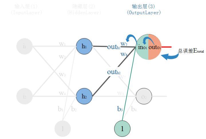
以权重$w_5$举例计算：权重$w$的大小能直接影响输出，$w$不合适会使输出有误差。要知道某个$w$对误差影响的程度，可以用误差对该$w$的变化率来表达。如果$w$的很少的变化，会导致误差增大很多，说明这个$w$对误差影响的程度就更大，也就是说，误差对该$w$的变化率越高。而误差对$w$的变化率就是误差对$w$的偏导。如图，总误差的大小首先受输出层神经元$O_1$的输出影响，继续反推，$O_1$的输出受它自己的输入的影响，而它自己的输入会受到$w_5$的影响。
那么根据链式法则有：$$\begin{aligned} \frac{\partial E_{total}}{\partial w_5}&=\frac{\partial E_{total}}{\partial OUT_{O_1}}\frac{\partial OUT_{O_1}}{\partial IN_{O_1}}\frac{\partial IN_{O_1}}{\partial w_5}\end{aligned} $$
第一部分： $$ \begin{aligned} \because E_{total}&=\frac{1}{2}(O_1-OUT_{O_1})^2+\frac{1}{2}(O_2-OUT_{O_2})^2 \\ \therefore \frac{\partial E_{total}}{\partial OUT_{O_1}}&=\frac{\partial (\frac{1}{2}(O_1-OUT_{O_1})^2+\frac{1}{2}(O_2-OUT_{O_2})^2)}{\partial OUT_{O_1}} \\ & =2\ast \frac{1}{2}(O_1-OUT_{O_1})^{2-1}\ast (0-1)+0 \\ & =-(O_1-OUT_{O_1}) \\ & =-(0.01-0.7987314002) \\ & =0.7887314002 \end{aligned}$$
第二部分：$$\begin{aligned}\because OUT_{O_1}&=\frac{1}{e^{-IN_{O_1}}+1} \\ \therefore \frac{\partial OUT_{O_1}}{\partial IN_{O_1}}&=\frac{\partial (\frac{1}{e^{-IN_{O_1}}+1})}{\partial IN_{O_1}} \\ & =OUT_{O_1}(1-OUT_{O_1}) \\ &=0.7987314002*(1-0.7987314002) \\ &=0.1607595505 \end{aligned}$$
第三部分：$$\begin{aligned} \because IN_{O_1}&=w_5\ast OUT_{h_1}+w_6\ast OUT_{h_2}+1\ast b_3 \\ \therefore \frac{\partial IN_{O_1}}{\partial w_5}&=\frac{\partial (w_5\ast OUT_{h_1}+w_6\ast OUT_{H}+1\ast b_3)}{\partial w_5} \\ &=1\ast w_5^{(1-1)}\ast OUT_{h_1}+0+0 \\ &=OUT_{h_1} \\ &=0.6456563062\end{aligned}$$
所以：$$\begin{aligned}\frac{\partial E_{total}}{\partial w_5}&=\frac{\partial E_{total}}{\partial OUT_{O_1}}\frac{\partial OUT_{O_1}}{\partial IN_{O_1}}\frac{\partial IN_{O_1}}{\partial w_5} \\ &=0.7887314002\ast 0.1607595505\ast 0.6456563062\\ &=0.0818667051\end{aligned}$$
归纳如下：$$\begin{aligned}\frac{\partial E_{total}}{\partial w_5}&=\frac{\partial E_{total}}{\partial OUT_{O_1}}\frac{\partial OUT_{O_1}}{\partial IN_{O_1}}\frac{\partial IN_{O_1}}{\partial w_5} \\ &=-(O_1-OUT_{O_1})\cdot OUT_{O_1}\cdot (1-OUT_{O_1})\cdot OUT_{h_1}\\ &=\sigma_{O_1}\cdot OUT_{h_1} \\ & 其中，\sigma_{O_1}=-(O_1-OUT_{O_1})\cdot OUT_{O_1}\cdot (1-OUT_{O_1})\end{aligned}$$

隐藏层–>输出层的偏置的更新：
同理输出层偏置b更新如下：$$\begin{aligned} IN_{O_1}&=w_5\ast OUT_{h_1}+w_6\ast OUT_{h_2}+1\ast b_3 \\ \frac{\partial IN_{O_1}}{\partial b_3}&=\frac{w_5\ast OUT_{h_1}+w_6\ast OUT_{h_2}+1\ast b_3}{\partial b_3} \\ &=0+0+b_3^{(1-1)} \\&=1 \end{aligned}$$
所以：$$\begin{aligned}\frac{\partial E_{total}}{\partial b_3}&=\frac{\partial E_{total}}{\partial OUT_{O_1}}\frac{\partial OUT_{O_1}}{\partial IN_{O_1}}\frac{\partial IN_{O_1}}{\partial b_3} \\ &=0.7887314002\ast 0.1607595505\ast 1\\ &=0.1267961053\end{aligned}$$
归纳如下： $$\begin{aligned} \frac{\partial E_{total}}{\partial b_3}&=\frac{\partial E_{total}}{\partial OUT_{O_1}}\frac{\partial OUT_{O_1}}{\partial IN_{O_1}}\frac{\partial IN_{O_1}}{\partial b_3}\\ &=-(O_1-OUT_{O_1})\cdot OUT_{O_1}\cdot (1-OUT_{O_1})\cdot 1\\ &=\sigma_{O_1}\\ &其中,\sigma_{O_1}=-(O_1-OUT_{O_1})\cdot OUT_{O_1}\cdot (1-OUT_{O_1}) \end{aligned}$$

更新$w_5$的值：

暂时设定学习率为0.5，学习率不宜过大也不宜过小，这篇文章学习率有更为详细的介绍，更新$w_5$：$$\begin{aligned}w_5^+&=w_5-\alpha \cdot \frac{\partial E_{total}}{\partial w_5} \\ &=0.5-0.5\ast 0.0818667051\\ &=0.45906664745\end{aligned}$$
同理可以计算出其他$w_n$的值
归纳输出层$w$的更新公式：$$\begin{aligned}w_O^+&=w_o-\alpha \cdot (-OUT_O\cdot (1-OUT_O)\cdot (O-OUT_O)\cdot OUT_h)\\ &=w_O+\alpha \cdot (O-OUT_O)\cdot OUT_O\cdot (1-OUT_O)\cdot OUT_h\end{aligned}$$

更新$b_3$的值：

更新偏置b：$$\begin{aligned}b_3^+&=b_{O_3}-\alpha \cdot \frac{\partial E_{total}}{\partial b_{O_3}} \\ &=0.66-0.5\cdot 0.1267961053\\ &=0.596601947 \end{aligned}$$
归纳如下：$$\begin{aligned}b_O^+&=b_O-\alpha \cdot(-OUT_O\cdot(1-OUT_O)\cdot(O_OUT_O))\\ &=b_O+\alpha \cdot (O-OUT_O)\cdot OUT_O\cdot(1-OUT_O)\end{aligned}$$

输入层–>隐藏层的权值更新：

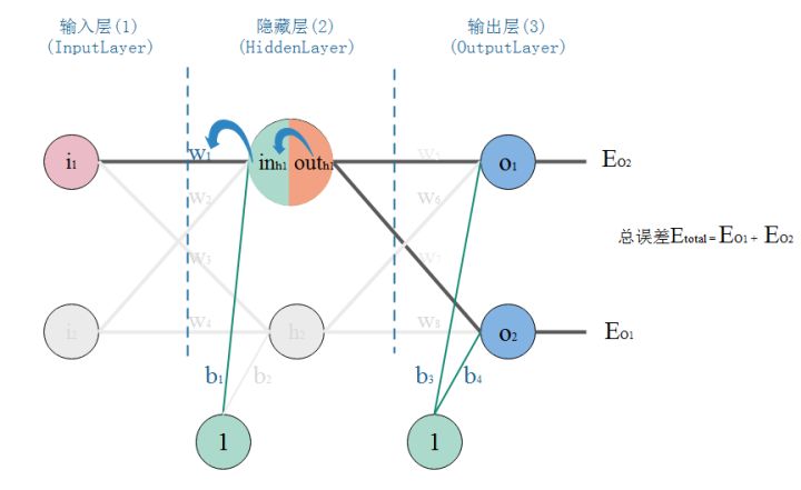
以权重$w_1$举例计算：在求$w_5$的更新，误差反向传递路径输出层–>隐层，即$OUT_{O_1}\rightarrow IN_{O_1}\rightarrow w_5$，总误差只有一条路径能传回来。但是求$w_1$时，误差反向传递路径是隐藏层–>输入层，但是隐藏层的神经元是有2条的，所以总误差沿着2个路径回来，也就是说，计算偏导时，要分开来算。

计算总误差对$w_1$的偏导：

$$
\begin{aligned}\frac{\partial E_{total}}{\partial w_1}&=\frac{\partial E_{total}}{\partial OUT_{h_1}}\cdot \frac{\partial OUT_{h_1}}{\partial IN_{h_1}}\cdot \frac{\partial IN_{h_1}}{\partial w_1} \\ &=(\frac{\partial E_{O_1}}{\partial OUT_{h_1}}+\frac{\partial E_{O_2}}{\partial OUT_{h_1}})\cdot \frac{\partial OUT_{h_1}}{\partial IN_{h_1}}\cdot \frac{\partial IN_{h_1}}{\partial w_1}\end{aligned}
$$

计算$E_{O_1}对OUT_{h_1}$的偏导：$$\begin{aligned}\frac{\partial E_{total}}{\partial OUT_{h_1}} &= \frac{\partial E_{O_1}}{\partial OUT_{h_1}}+\frac{\partial E_{O_2}}{\partial OUT_{h_1}}\\ \frac{\partial E_{O_1}}{\partial OUT_{h_1}}&=\frac{\partial E_{O_1}}{\partial IN_{O_1}}\cdot\frac{\partial IN_{O_1}}{\partial OUT_{h_1}} \\ (左边)\frac{\partial E_{O_1}}{\partial IN_{O_1}}&=\frac{\partial E_{O_1}}{\partial OUT_{O_1}}\cdot\frac{\partial OUT_{O_1}}{\partial IN_{O_1}}\\ &=\frac{\frac{1}{2}(O_1-OUT_{O_1})^2}{\partial OUT_{O_1}}\cdot \frac{\partial OUT_{O_1}}{\partial IN_{O_1}}\\ &=-(O_1-OUT_{O_1})\cdot \frac{\partial OUT_{O_1}}{\partial IN_{O_1}}\\ &=0.7987314002\ast 0.1607595505\\ &=0.1284037009\\IN_{O_1}&=w_5\ast OUT_{h_1}+w_6\ast OUT_{h_2}+1\ast b_3\\ (右边)\frac{\partial IN_{O_1}}{\partial OUT_{h_1}}&=\frac{\partial (w_5\ast OUT_{h_1}+w_6\ast OUT_{h_2}+1\ast b_3)}{\partial OUT_{h_1}}\\ &=w_5\ast OUT_{h_1}^{(1-1)}+0+0\\ &=w_5=0.5 \\ \frac{\partial E_{O_1}}{\partial OUT_{h_1}} &=\frac{\partial E_{O_1}}{\partial IN_{O_1}}\cdot \frac{\partial IN_{O_1}}{\partial OUT_{h_1}}\\ &=0.1284037009\ast 0.5=0.06420185045\end{aligned}$$
j计算$E_{O_2}对OUT_{h_1}$的偏导：$$\begin{aligned}\frac{\partial E_{O_2}}{\partial OUT_{h_1}}&=\frac{\partial E_{O_2}}{\partial IN_{O_2}}\cdot\frac{\partial IN_{O_2}}{\partial OUT_{h_1}}\\ &=-(O_2-OUT_{O_2})\cdot \frac{\partial OUT_{O_2}}{\partial IN_{O_2}}\cdot \frac{\partial IN_{O_2}}{\partial OUT_{h_1}}\\ &=-(O_2-OUT_{O_2})\cdot OUT_{O_2}(1-OUT_{O_2})\cdot w_7\\ &=-(0.99-0.8374488853)\ast 0.8374488853\ast (1-0.8374488853)\ast 0.7=-0.0145365614\end{aligned}$$
则$E_{total}对OUT_{h_1}$的偏导为：$$\begin{aligned}\frac{\partial E_{total}}{\partial OUT_{h_1}} &= \frac{\partial E_{O_1}}{\partial OUT_{h_1}}+\frac{\partial E_{O_2}}{\partial OUT_{h_1}}\\ &=0.06420185045+(-0.0145365614)=0.04966528905\end{aligned}$$
计算$OUT_{h_1}$对$IN_{h_1}$的偏导：$$\begin{aligned}\because OUT_{h_1}&=\frac{1}{e^{-IN_{h_1}}+1} \\ \therefore \frac{\partial OUT_{h_1}}{\partial IN_{h_1}}&= \frac{\partial (\frac{1}{e^{-IN_{h_1}}+1})}{\partial IN_{h_1}} \\ &=OUT(1-OUT_{h_1})\\ &=0.6456563062\ast (1-0.6456563062)=0.2298942405 \end{aligned}$$
计算$IN_{h_1}对w_1$的偏导：$$\begin{aligned}\frac{\partial IN_{h_1}}{\partial w_1}&=\frac{\partial(w_1\ast i_1+w_2\ast i_2+1\ast b)}{\partial w_1}\\ &=w_1^{(1-1)}\ast i_1+0+0=i_1=0.1\end{aligned}$$
三者相乘计算$E_{total}$对$w_1$的偏导：$$\begin{aligned}\frac{\partial E_{total}}{\partial w_1}&=\frac{\partial E_{total}}{\partial OUT_{h_1}}\cdot \frac{\partial OUT_{h_1}}{\partial IN_{h_1}}\cdot \frac{\partial IN_{h_1}}{\partial w_1}\\ &=0.04966528905\ast 0.2298942405\ast 0.1=0.0011362635\end{aligned}$$
归纳：$$\begin{aligned}\frac{\partial E_{total}}{\partial w_1}&=\frac{\partial E_{total}}{\partial OUT_{h_1}}\cdot \frac{\partial OUT_{h_1}}{\partial IN_{h_1}}\cdot \frac{\partial IN_{h_1}}{\partial w_1}\\ &=(\frac{\partial E_{O_1}}{\partial OUT_{h_1}}+\frac{\partial E_{O_2}}{\partial OUT_{h_1}})\cdot \frac{\partial OUT_{h_1}}{\partial IN_{h_1}}\cdot \frac{\partial IN_{h_1}}{\partial w_1}\\ &=(\sum_{n=1}^2\frac{\partial E_{O_n}}{\partial OUT_{O_n}}\cdot\frac{\partial OUT_{O_n}}{\partial IN_{O_n}}\cdot \frac{\partial IN_{O_n}}{\partial OUT_{h_n}})\cdot \frac{\partial OUT_{h_1}}{\partial IN_{h_1}}\cdot \frac{\partial IN_{h_1}}{\partial w_1}\\ &=(\sum_{n=1}^2\sigma_{O_n}w_{O_n})\cdot OUT_{h_n}(1-OUT_{h_n})\cdot i_1\\ &=\sigma_{h_1}\cdot i_1\\&其中，\sigma_{h_1}=(\sum_{n=1}^2\sigma_{O_n}w_{O_n})\cdot OUT_{h_1}(1-OUT_{h_1})\\&\sigma_{O_i}看作输出层的误差，误差和w相乘，相当于通过w传播了过来；如果是深层网络，隐藏层数量>1，那么公式中的\sigma_{O_n}写为\sigma_{h_n}，w_O写成w_h\end{aligned}$$
现在更新$w_1$的值：$$\begin{aligned}w_1^+&=w_1-\alpha\cdot \frac{\partial E_{total}}{\partial w_1}\\ &=0.1-0.1\ast 0.0011362635=0.0998863737\end{aligned}$$
归纳隐藏层$w$更新的公式：$$\begin{aligned}w_h^+&=w_h-\alpha\cdot \frac{\partial E_{total}}{\partial w}\\ &=w_h+\alpha\cdot (-\sum_{n=1}^2\sigma_{O_n}w_{O_n})\cdot OUT_{h_n}(1-OUT_{h_n})\cdot i_1\end{aligned}$$
计算隐藏层偏置b的更新：

$$
\begin{aligned}\frac{\partial E_{total}}{\partial b_h}&=(\sum_h\sigma_hw_h)\cdot OUT_h(1-OUT_h)\\ b_h^+&=b_h-\alpha\cdot \frac{\partial E_{total}}{\partial b_n}\\ &=w_h+\alpha\cdot (\sum_h\sigma_hw_h)\cdot OUT_h(1-OUT_h)\end{aligned}
$$

代码实现

#coding:utf-8
import h5py
import sklearn.datasets
import sklearn.linear_model
import matplotlib
import matplotlib.font_manager as fm
import matplotlib.pyplot as plt
import numpy as np

np.random.seed(1)

font = fm.FontProperties(fname='/System/Library/Fonts/STHeiti Light.ttc')
matplotlib.rcParams['figure.figsize'] = (10.0, 8.0)

def sigmoid(input_sum):

    """

    函数：
        激活函数Sigmoid
    输入：
        input_sum: 输入，即神经元的加权和
    返回：

        output: 激活后的输出
        input_sum: 把输入缓存起来返回
    """

    output = 1.0/(1+np.exp(-input_sum))
    return output, input_sum



def sigmoid_back_propagation(derror_wrt_output, input_sum):
    """
    函数：
        误差关于神经元输入的偏导: dE／dIn = dE/dOut * dOut/dIn  参照式（5.6）
        其中： dOut/dIn 就是激活函数的导数 dy=y(1 - y)，见式（5.9）
              dE/dOut 误差对神经元输出的偏导，见式（5.8）
    输入：
        derror_wrt_output：误差关于神经元输出的偏导: dE/dyⱼ = 1/2(d(expect_to_output - output)**2/doutput) = -(expect_to_output - output)
        input_sum: 输入加权和
    返回：
        derror_wrt_dinputs: 误差关于输入的偏导，见式（5.13）
    """
    output = 1.0/(1 + np.exp(- input_sum))
    doutput_wrt_dinput = output * (1 - output)
    derror_wrt_dinput =  derror_wrt_output * doutput_wrt_dinput
    return derror_wrt_dinput


def relu(input_sum):

    """
        函数：
            激活函数ReLU
        输入：
            input_sum: 输入，即神经元的加权和
        返回：
            outputs: 激活后的输出
            input_sum: 把输入缓存起来返回
    """

    output = np.maximum(0, input_sum)
    return output, input_sum


def relu_back_propagation(derror_wrt_output, input_sum):

    """
        函数：
            误差关于神经元输入的偏导: dE／dIn = dE/dOut * dOut/dIn
            其中： dOut/dIn 就是激活函数的导数
                  dE/dOut 误差对神经元输出的偏导
        输入：
            derror_wrt_output：误差关于神经元输出的偏导
            input_sum: 输入加权和
        返回：
            derror_wrt_dinputs: 误差关于输入的偏导
    """

    derror_wrt_dinputs = np.array(derror_wrt_output, copy=True)
    derror_wrt_dinputs[input_sum <= 0] = 0

    return derror_wrt_dinputs


def tanh(input_sum):

    """
    函数：
        激活函数 tanh
    输入：
        input_sum: 输入，即神经元的加权和
    返回：
        output: 激活后的输出
        input_sum: 把输入缓存起来返回
    """
    output = np.tanh(input_sum)
    return output, input_sum


def tanh_back_propagation(derror_wrt_output, input_sum):

    """
    函数：
        误差关于神经元输入的偏导: dE／dIn = dE/dOut * dOut/dIn
        其中： dOut/dIn 就是激活函数的导数 tanh'(x) = 1 - x²
              dE/dOut 误差对神经元输出的偏导
    输入：
        derror_wrt_output：误差关于神经元输出的偏导: dE/dyⱼ = 1/2(d(expect_to_output - output)**2/doutput) = -(expect_to_output - output)
        input_sum: 输入加权和
    返回：
        derror_wrt_dinputs: 误差关于输入的偏导
    """

    output = np.tanh(input_sum)
    doutput_wrt_dinput = 1 - np.power(output, 2)
    derror_wrt_dinput =  derror_wrt_output * doutput_wrt_dinput

    return derror_wrt_dinput


def activated(activation_choose, input):

    """把正向激活包装一下"""
    if activation_choose == "sigmoid":
        return sigmoid(input)
    elif activation_choose == "relu":
        return relu(input)
    elif activation_choose == "tanh":
        return tanh(input)

    return sigmoid(input)


def activated_back_propagation(activation_choose, derror_wrt_output, output):
    """包装反向激活传播"""
    if activation_choose == "sigmoid":
        return sigmoid_back_propagation(derror_wrt_output, output)
    elif activation_choose == "relu":
        return relu_back_propagation(derror_wrt_output, output)
    elif activation_choose == "tanh":
        return tanh_back_propagation(derror_wrt_output, output)

    return sigmoid_back_propagation(derror_wrt_output, output)

class NeuralNetwork:

    def __init__(self, layers_strcuture, print_cost = False):
        self.layers_strcuture = layers_strcuture
        self.layers_num = len(layers_strcuture)

        # 除掉输入层的网络层数，因为其他层才是真正的神经元层
        self.param_layers_num = self.layers_num - 1

        self.learning_rate = 0.0618
        self.num_iterations = 2000
        self.x = None
        self.y = None
        self.w = dict()
        self.b = dict()
        self.costs = []
        self.print_cost = print_cost

        self.init_w_and_b()

    def set_learning_rate(self, learning_rate):
        """设置学习率"""
        self.learning_rate = learning_rate

    def set_num_iterations(self, num_iterations):
        """设置迭代次数"""
        self.num_iterations = num_iterations

    def set_xy(self, input, expected_output):
        """设置神经网络的输入和期望的输出"""
        self.x = input
        self.y = expected_output

    def init_w_and_b(self):

        """
        函数:
            初始化神经网络所有参数
        输入:
            layers_strcuture: 神经网络的结构，例如[2,4,3,1]，4层结构:
                第0层输入层接收2个数据，第1层隐藏层4个神经元，第2层隐藏层3个神经元，第3层输出层1个神经元
        返回: 神经网络各层参数的索引表，用来定位权值 wᵢ  和偏置 bᵢ，i为网络层编号
        """
        np.random.seed(3)

        # 当前神经元层的权值为 n_i x n_(i-1)的矩阵，i为网络层编号，n为下标i代表的网络层的节点个数
        # 例如[2,4,3,1]，4层结构：第0层输入层为2，那么第1层隐藏层神经元个数为4
        # 那么第1层的权值w是一个 4x2 的矩阵，如：
        #    w1 = array([ [-0.96927756, -0.59273074],
        #                 [ 0.58227367,  0.45993021],
        #                 [-0.02270222,  0.13577601],
        #                 [-0.07912066, -1.49802751] ])
        # 当前层的偏置一般给0就行，偏置是个1xnᵢ的矩阵，nᵢ为第i层的节点个数，例如第1层为4个节点，那么：
        #    b1 = array([ 0.,  0.,  0.,  0.])



        for l in range(1, self.layers_num):
            self.w["w" + str(l)] = np.random.randn(self.layers_strcuture[l], self.layers_strcuture[l-1])/np.sqrt(self.layers_strcuture[l-1])
            self.b["b" + str(l)] = np.zeros((self.layers_strcuture[l], 1))
        return self.w, self.b

    def layer_activation_forward(self, x, w, b, activation_choose):

        """
        函数：
            网络层的正向传播
        输入：
            x: 当前网络层输入（即上一层的输出），一般是所有训练数据，即输入矩阵
            w: 当前网络层的权值矩阵
            b: 当前网络层的偏置矩阵
            activation_choose: 选择激活函数 "sigmoid", "relu", "tanh"
        返回:
            output: 网络层的激活输出
            cache: 缓存该网络层的信息，供后续使用： (x, w, b, input_sum) -> cache
     """

        # 对输入求加权和，见式（5.1）
        input_sum = np.dot(w, x) + b

        # 对输入加权和进行激活输出
        output, _ = activated(activation_choose, input_sum)

        return output, (x, w, b, input_sum)



    def forward_propagation(self, x):
        """
        函数:
            神经网络的正向传播
        输入:

        返回:
            output: 正向传播完成后的输出层的输出
            caches: 正向传播过程中缓存每一个网络层的信息： (x, w, b, input_sum),... -> caches
        """
        caches = []

        #作为输入层，输出 = 输入
        output_prev = x

        #第0层为输入层，只负责观察到输入的数据，并不需要处理，正向传播从第1层开始，一直到输出层输出为止

        # range(1, n) => [1, 2, ..., n-1]
        L = self.param_layers_num
        for l in range(1, L):

            # 当前网络层的输入来自前一层的输出
            input_cur = output_prev
            output_prev, cache = self.layer_activation_forward(input_cur, self.w["w"+ str(l)], self.b["b" + str(l)], "tanh")
            caches.append(cache)



        output, cache = self.layer_activation_forward(output_prev, self.w["w" + str(L)], self.b["b" + str(L)], "sigmoid")
        caches.append(cache)

        return output, caches

    def show_caches(self, caches):
        """显示网络层的缓存参数信息"""
        i = 1
        for cache in caches:
            print("%dtd Layer" % i)
            print(" input: %s" % cache[0])
            print(" w: %s" % cache[1])
            print(" b: %s" % cache[2])
            print(" input_sum: %s" % cache[3])
            print("----------")
            i += 1

    def compute_error(self, output):
        """
        函数:
            计算档次迭代的输出总误差
        输入:
        返回:

        """

        m = self.y.shape[1]

        # 计算误差，见式(5.5): E = Σ1/2(期望输出-实际输出)²
        #error = np.sum(0.5 * (self.y - output) ** 2) / m
        # 交叉熵作为误差函数

        error =  -np.sum(np.multiply(np.log(output),self.y) + np.multiply(np.log(1 - output), 1 - self.y)) / m
        error = np.squeeze(error)

        return error



    def layer_activation_backward(self, derror_wrt_output, cache, activation_choose):

        """
            函数:
                网络层的反向传播
            输入:
                derror_wrt_output: 误差关于输出的偏导
                cache: 网络层的缓存信息 (x, w, b, input_sum)
                activation_choose: 选择激活函数 "sigmoid", "relu", "tanh"
            返回: 梯度信息，即
                derror_wrt_output_prev: 反向传播到上一层的误差关于输出的梯度
                derror_wrt_dw: 误差关于权值的梯度
                derror_wrt_db: 误差关于偏置的梯度
        """

        input, w, b, input_sum = cache
        output_prev = input     # 上一层的输出 = 当前层的输入; 注意是'输入'不是输入的加权和（input_sum）
        m = output_prev.shape[1]      # m是输入的样本数量，我们要取均值，所以下面的求值要除以m


        # 实现式（5.13）-> 误差关于权值w的偏导数
        derror_wrt_dinput = activated_back_propagation(activation_choose, derror_wrt_output, input_sum)
        derror_wrt_dw = np.dot(derror_wrt_dinput, output_prev.T) / m

        # 实现式 （5.32）-> 误差关于偏置b的偏导数
        derror_wrt_db = np.sum(derror_wrt_dinput, axis=1, keepdims=True)/m

        # 为反向传播到上一层提供误差传递，见式（5.28）的 （Σδ·w） 部分
        derror_wrt_output_prev = np.dot(w.T, derror_wrt_dinput)

        return derror_wrt_output_prev, derror_wrt_dw, derror_wrt_db

    def back_propagation(self, output, caches):

        """
        函数:
            神经网络的反向传播
        输入:
            output：神经网络输
            caches：所有网络层（输入层不算）的缓存参数信息  [(x, w, b, input_sum), ...]
        返回:
            grads: 返回当前迭代的梯度信息
        """

        grads = {}
        L = self.param_layers_num #
        output = output.reshape(output.shape)  # 把输出层输出输出重构成和期望输出一样的结构

        expected_output = self.y

        # 见式(5.8)
        #derror_wrt_output = -(expected_output - output)

        # 交叉熵作为误差函数
        derror_wrt_output = - (np.divide(expected_output, output) - np.divide(1 - expected_output, 1 - output))

        # 反向传播：输出层 -> 隐藏层，得到梯度：见式(5.8), (5.13), (5.15)
        current_cache = caches[L - 1] # 取最后一层,即输出层的参数信息
        grads["derror_wrt_output" + str(L)], grads["derror_wrt_dw" + str(L)], grads["derror_wrt_db" + str(L)] = \
            self.layer_activation_backward(derror_wrt_output, current_cache, "sigmoid")

        # 反向传播：隐藏层 -> 隐藏层，得到梯度：见式 (5.28)的(Σδ·w), (5.28), (5.32)
        for l in reversed(range(L - 1)):
            current_cache = caches[l]
            derror_wrt_output_prev_temp, derror_wrt_dw_temp, derror_wrt_db_temp = \
                self.layer_activation_backward(grads["derror_wrt_output" + str(l + 2)], current_cache, "tanh")

            grads["derror_wrt_output" + str(l + 1)] = derror_wrt_output_prev_temp
            grads["derror_wrt_dw" + str(l + 1)] = derror_wrt_dw_temp
            grads["derror_wrt_db" + str(l + 1)] = derror_wrt_db_temp

        return grads



    def update_w_and_b(self, grads):
        """
        函数:
            根据梯度信息更新w，b
        输入:
            grads：当前迭代的梯度信息
        返回:

        """

        # 权值w和偏置b的更新，见式:（5.16),(5.18)
        for l in range(self.param_layers_num):
            self.w["w" + str(l + 1)] = self.w["w" + str(l + 1)] - self.learning_rate * grads["derror_wrt_dw" + str(l + 1)]
            self.b["b" + str(l + 1)] = self.b["b" + str(l + 1)] - self.learning_rate * grads["derror_wrt_db" + str(l + 1)]

    def training_modle(self):
        """训练神经网络模型"""

        np.random.seed(5)
        for i in range(0, self.num_iterations):
            # 正向传播，得到网络输出，以及每一层的参数信息
            output, caches = self.forward_propagation(self.x)

            # 计算网络输出误差
            cost = self.compute_error(output)

            # 反向传播，得到梯度信息
            grads = self.back_propagation(output, caches)

            # 根据梯度信息，更新权值w和偏置b
            self.update_w_and_b(grads)

            # 当次迭代结束，打印误差信息
            if self.print_cost and i % 1000 == 0:
                print ("Cost after iteration %i: %f" % (i, cost))
            if self.print_cost and i % 1000 == 0:
                self.costs.append(cost)

        # 模型训练完后显示误差曲线
        if False:
            plt.plot(np.squeeze(self.costs))
            plt.ylabel(u'神经网络误差', fontproperties = font)
            plt.xlabel(u'迭代次数 (*100)', fontproperties = font)
            plt.title(u"学习率 =" + str(self.learning_rate), fontproperties = font)
            plt.show()

        return self.w, self.b

    def predict_by_modle(self, x):
        """使用训练好的模型（即最后求得w，b参数）来决策输入的样本的结果"""
        output, _ = self.forward_propagation(x.T)
        output = output.T
        result = output / np.sum(output, axis=1, keepdims=True)
        return np.argmax(result, axis=1)

def plot_decision_boundary(xy, colors, pred_func):
    # xy是坐标点的集合，把集合的范围算出来
    # 加减0.5相当于扩大画布的范围，不然画出来的图坐标点会落在图的边缘，逼死强迫症患者
    x_min, x_max = xy[:, 0].min() - 0.5, xy[:, 0].max() + 0.5
    y_min, y_max = xy[:, 1].min() - 0.5, xy[:, 1].max() + 0.5

    # 以h为分辨率，生成采样点的网格，就像一张网覆盖所有颜色点
    h = .01
    xx, yy = np.meshgrid(np.arange(x_min, x_max, h), np.arange(y_min, y_max, h))

    # 把网格点集合作为输入到模型，也就是预测这个采样点是什么颜色的点，从而得到一个决策面
    Z = pred_func(np.c_[xx.ravel(), yy.ravel()])
    Z = Z.reshape(xx.shape)

    # 利用等高线，把预测的结果画出来，效果上就是画出红蓝点的分界线
    plt.contourf(xx, yy, Z, cmap=plt.cm.Spectral)

    # 训练用的红蓝点点也画出来
    plt.scatter(xy[:, 0], xy[:, 1], c=colors, marker='o', cmap=plt.cm.Spectral, edgecolors='black')


if __name__ == "__main__":
    plt.figure(figsize=(16, 32))

    # 用sklearn的数据样本集，产生2种颜色的坐标点，noise是噪声系数，噪声越大，2种颜色的点分布越凌乱
    xy, colors = sklearn.datasets.make_moons(60, noise=1.0)

    # 因为点的颜色是1bit，我们设计一个神经网络，输出层有2个神经元。
    # 标定输出[1,0]为红色点，输出[0,1]为蓝色点
    expect_output = []
    for c in colors:
        if c == 1:
            expect_output.append([0,1])
        else:
            expect_output.append([1,0])

    expect_output = np.array(expect_output).T

    # 设计3层网络，改变隐藏层神经元的个数，观察神经网络分类红蓝点的效果
    hidden_layer_neuron_num_list = [1,2,4,10,20,50]

    for i, hidden_layer_neuron_num in enumerate(hidden_layer_neuron_num_list):
        plt.subplot(5, 2, i + 1)
        plt.title(u'隐藏层神经元数量: %d' % hidden_layer_neuron_num, fontproperties = font)

        nn = NeuralNetwork([2, hidden_layer_neuron_num, 2], True)

        # 输出和输入层都是2个节点，所以输入和输出的数据集合都要是 nx2的矩阵
        nn.set_xy(xy.T, expect_output)
        nn.set_num_iterations(30000)
        nn.set_learning_rate(0.1)
        w, b = nn.training_modle()
        plot_decision_boundary(xy, colors, nn.predict_by_modle)

    plt.show()

本博客所有文章除特别声明外，均采用 CC BY-SA 4.0 协议，转载请注明出处！

机器学习的数学基础上一篇

自动微分法下一篇

BP神经网络原理和简明理解